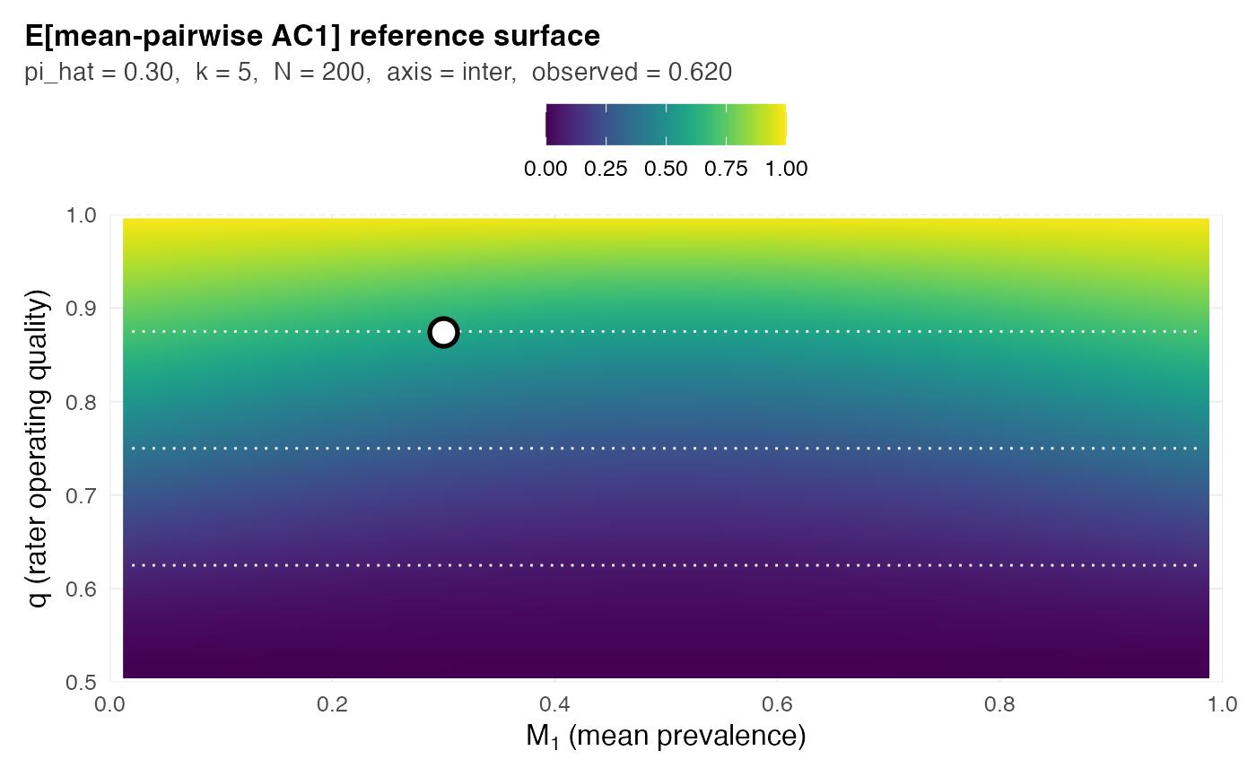
Standalone reference-surface plot for prospective study design

Renders the same context-conditioned reference surface that plot.grass_card(type = "surface") shows, but driven by scalar inputs rather than a fitted grass_report() result. The intended use case is prospective study design: a practitioner planning a multi-rater study at design (pi_hat, k, N) can ask "what does my reference surface look like for this metric, before I collect data?" – and plot_surface() answers without requiring a rating matrix.

Usage

plot_surface(
  metric,
  pi_hat = NULL,
  observed = NULL,
  k = NULL,
  N = NULL,
  axis = c("inter", "intra"),
  bands = c(0.5, 0.625, 0.75, 0.875, 1),
  ...
)

Arguments

metric

Character scalar. One of "pabak", "mean_pabak", "fleiss_kappa", "kappa", "mean_ac1", "ac1", "krippendorff_a". ICC is not supported (see Details).

pi_hat

Optional numeric scalar in (0, 1). The design's marginal positive rate. If supplied alone, draws a vertical reference line on the surface; if supplied together with observed, anchors the pin point.

observed

Optional numeric scalar. An observed (or hypothetical) coefficient value. When supplied with pi_hat, the function inverts to hat q and pins a marker at (pi_hat, hat q).

k

Optional integer. Rater count. Used for the subtitle only; non-ICC closed-form surfaces are k-invariant.

N

Optional integer. Sample size. Used for the subtitle only; non-ICC closed-form surfaces are N-invariant in the large-N limit the surface represents.

axis

One of "inter" (default) or "intra". Used for the subtitle only.

bands

Numeric length-5 vector giving band boundaries on q. Default c(0.5, 0.625, 0.75, 0.875, 1.0).

...

Reserved for future extension.

Value

A ggplot object.

Details

The plot is a heatmap of the closed-form expectation E[metric](M_1, q) over the surface, where M_1 is the marginal positive rate and q in [0.5, 1] is the diagonal rater operating quality. Dotted contours overlay the four-band partition (bands argument). When pi_hat is supplied alone, a dashed vertical line marks the design's marginal. When both pi_hat and observed are supplied, a filled marker pins the implied (M_1, hat q) point on the surface; hat q is recovered by closed-form inversion of observed against the reference curve at pi_hat.

This function uses the closed-form non-ICC surfaces only (PABAK, Fleiss kappa, mean-pairwise AC1, Krippendorff alpha). ICC surfaces depend on the full subject-prevalence distribution F and the GLMM-gap-corrected fitted reference; those are accessed via position_on_surface() with metric = "icc" and (if available) a fitted card via plot.grass_card(type = "surface").

See also

plot.grass_card() for the card-driven surface view that adds card-specific annotations (band, qualifier, primary-coefficient pin); position_on_surface() for the underlying inversion machinery.

Examples

# \donttest{
if (requireNamespace("ggplot2", quietly = TRUE)) {
  # Bare surface -- what does PABAK's reference look like?
  plot_surface("pabak")

  # Mark a design context (no observed value yet -- pre-data).
  plot_surface("fleiss_kappa", pi_hat = 0.30, k = 5, N = 200)

  # Pin a hypothetical observation on the surface.
  plot_surface("mean_ac1", pi_hat = 0.30, observed = 0.62,
               k = 5, N = 200)
}
#> Warning: The following aesthetics were dropped during statistical transformation: fill.
#> ℹ This can happen when ggplot fails to infer the correct grouping structure in
#>   the data.
#> ℹ Did you forget to specify a `group` aesthetic or to convert a numerical
#>   variable into a factor?
#> Warning: Removed 120 rows containing missing values or values outside the scale range
#> (`geom_raster()`).

# }