grassr: rater reliability on binary outcomes, from rating matrix to Report Card

Austin Semmel

Rachel Gidaro

2026-09-06

Introduction: the prevalence trap

In a study protocol where a rater panel of k members evaluates N subjects on a binary outcome, the resulting N x k response matrix is traditionally assessed against fixed benchmarks such as the Landis and Koch (1977) kappa scale. However, these classical metrics are vulnerable to prevalence skew, rater count, and sample size, and can label identical rater performance as either slight or substantial purely because of the base rate. grassr (Guide for Rater Agreement under Structural Skew) resolves this prevalence trap by simulating panels within your study’s specific context, translating raw coefficients into an empirical Report Card that reports a percentile for each coefficient, a consistency band on rater quality, and a flag when the coefficients disagree.

The code below fixes two raters at quality 0.87, meaning each calls 87% of cases correctly, sweeps prevalence from 2% to 98%, and plots the expected Cohen’s kappa against the Landis and Koch bands.

q <- 0.87                       # every rater calls 87% of cases correctly
prev <- seq(0.02, 0.98, 0.005)
Pa <- q^2 + (1 - q)^2           # P(two such raters agree); prevalence-free
pip <- prev * q + (1 - prev) * (1 - q)  # observed positive rate
kappa <- (Pa - (pip^2 + (1 - pip)^2)) / (1 - (pip^2 + (1 - pip)^2))

op <- par(mar = c(4.2, 4.2, 2.4, 1))
plot(prev, kappa, type = "l", lwd = 2, ylim = c(0, 0.8),
     xlab = "prevalence of the finding", ylab = "expected Cohen's kappa",
     main = "Same raters (q = 0.87) at every prevalence")
abline(h = c(0.20, 0.40, 0.60), lty = 3, col = "grey55")
text(rep(0.99, 4), c(0.10, 0.30, 0.50, 0.70), adj = 1, col = "grey40",
     cex = 0.8, labels = c("slight", "fair", "moderate", "substantial"))
pts <- c(0.05, 0.50, 0.90)
ptk <- sapply(pts, function(p) {
  pp <- p * q + (1 - p) * (1 - q)
  (Pa - (pp^2 + (1 - pp)^2)) / (1 - (pp^2 + (1 - pp)^2))
})
points(pts, ptk, pch = 19)
text(pts, ptk + 0.05, sprintf("%.2f", ptk), cex = 0.85)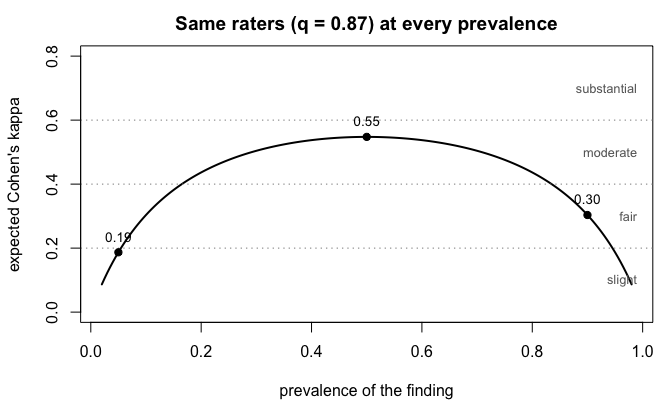

One panel of raters, three published verdicts.

par(op)

A screening study at 5% prevalence reports slight, a balanced study reports moderate, a high-prevalence study reports fair, and the raters never changed.

Quick start: the GRASS Report Card

The input is one matrix or data frame, subjects in rows and raters in columns, with at least two raters. Cells are numeric 0/1, logical, or a two-level factor or character column, where 1, TRUE, or the positive level means present. For a factor or character column the level named yes, true, positive, present, or case, in any letter case, is taken as positive; any other pair of labels is refused with a message asking for a 0/1 recode, so an outcome is never inverted silently. Drop identifier columns before the call. Column names, if given, become rater labels on the card. The functions stop on NA rather than silently dropping rows, so filter first with Y <- Y[complete.cases(Y), ] and report the exclusions in your Methods. Binary outcomes only.

The examples simulate the panel, so the true classes are known and every claim below can be checked against them. This first panel has 150 subjects at 30% prevalence and three raters who each call 87% of cases correctly.

library(grassr)
set.seed(7)
truth <- rbinom(150, 1, 0.30)                  # the latent true classes
Y0 <- sapply(1:3, function(j)                  # three raters, 87% accurate
  ifelse(truth == 1, rbinom(150, 1, 0.87), rbinom(150, 1, 0.13)))
colnames(Y0) <- c("R1", "R2", "R3")
head(Y0, 8)
#>      R1 R2 R3
#> [1,]  1  0  1
#> [2,]  0  0  0
#> [3,]  0  0  1
#> [4,]  0  0  0
#> [5,]  0  0  0
#> [6,]  1  1  1
#> [7,]  0  0  0
#> [8,]  1  1  0

Row 6 is unanimously positive, rows 2, 4, 5, and 7 unanimously negative, and rows 1, 3, and 8 split. One call produces the card. Inside a script, assign the result and print() it; the same goes for plot().

grass_report(ratings = Y0)
#> GRASS Report Card
#> 
#>   sample      = 3 raters, N = 150, pi_hat = 0.36
#>   PABAK        = 0.52  ->  70th percentile | quality 0.80-0.90  <- primary
#>   AC1          = 0.55  ->  70th percentile | quality 0.80-0.90
#>   Fleiss kappa = 0.48  ->  71st percentile | quality 0.80-0.90
#>   ICC          = 0.62  ->  72nd percentile | quality 0.81-0.90  [distribution-sensitive]
#>   read: this panel's agreement exceeds 70% of what panels in this study context can produce; the data are consistent with panel quality 0.80-0.90.
#>   delta       = 0.00 pp implied-quality spread (aligned)
#>   matched null = (k=3, N=150, q=0.86): delta_hat sits at percentile 11.6 of the null
#> 
#>   Notes:
#>     - ICC reference only: N=150 uses the nearest calibrated N=100. The agreement-family surfaces and the delta_hat null interpolate at N=150.
#>     - delta_hat is the implied-quality spread over the agreement family (PABAK, mean AC1, Fleiss kappa). ICC is shown but not included in delta_hat; its reference depends on how positive probability is spread across subjects, while the other three depend only on prevalence and quality.
#>     - flag from delta_hat's percentile on the matched null (k=3, N=150, q=0.86, prev=0.31; 50,000 draws); null interpolated between calibrated grid nodes.
#> 
#>   See `summary(...)` for full panel and CI details.
#>   See `plot(...)` for a surface-position visualization.

• sample is the study: rater count k, subject count N, and the observed positive rate pi_hat, the share of all N x k ratings that are positive. Here pi_hat is 0.36 against a true prevalence of 0.30, because false positives on the many negatives outnumber misses on the few positives. Together these three are the study context, the setting every reference panel is simulated in.
• The coefficient lines show each observed value, its percentile, and its consistency band. The percentile is where the observed value falls among everything this study could have produced, from the lowest-quality panels in the reference to the highest. Panel quality q is the share of cases a rater gets correct. The reference panels give every rater the same q for both sensitivity and specificity, and q is what the package is estimating. The consistency band is the range of qualities that could plausibly have produced this coefficient. Formally, it is every q at which the observed value sits inside the middle 95% of that quality’s panels. A wide band means the study cannot tell those qualities apart, and a small study always gives a wide band.
• <- primary marks the coefficient to report: PABAK (prevalence-adjusted bias-adjusted kappa; Byrt, Bishop, and Carlin,
  1993. at moderate prevalence, AC1 (Gwet, 2008) when the positive rate is below 0.15 or above 0.85 (0.20 or 0.80 at two raters), where its percentile is less noisy. The intraclass correlation coefficient (ICC) is tagged [distribution-sensitive] because its reference depends on how the positives are spread across subjects, a few obvious cases or many borderline ones, and not just on how many there are, so its percentile is less certain than the other three.
• The read: line restates the headline in plain language. The card prints no verdict label, and the band’s width states the uncertainty.
• delta is delta_hat as the card prints it, the spread of the qualities implied by PABAK, AC1 (both averaged over rater pairs), and Fleiss’ kappa, in percentage points (pp), followed by its flag. The next section covers the flag.

Intra-rater agreement, one rater scoring the same subjects on repeated occasions, uses the same layout with the occasions as columns and the call grass_report(Y, axis = "intra"). The same reference applies, since a rater re-reading the same subjects is modeled exactly like independent raters of equal quality, and the card has the same fields. On this axis the card marks ICC as primary, the conventional intra-rater statistic; the three agreement coefficients still print and still feed delta_hat. The card’s note says which way the two departures from that model push the reading: drift between occasions lowers it, and memory of an earlier pass raises it.

When coefficients disagree: the delta_hat flag

Every coefficient on the card can be turned back into a panel quality. PABAK has a formula, q_hat = (1 + sqrt(PABAK)) / 2; the others are looked up on their reference surfaces. delta_hat is the gap between the highest and lowest of those qualities across PABAK, AC1, and Fleiss’ kappa, in percentage points of quality, so a spread of 0.42 pp is 0.0042 on the 0-to-1 quality scale. ICC is left out because its reference depends on more than prevalence and quality.

Some spread happens by chance even when every rater is equally good, so the observed spread is compared with what equal-quality panels produce at the same rater count, sample size, quality, and prevalence. That is the matched null, and the card prints which cell it used. Below the null’s 95th percentile the flag is aligned, from the 95th caution, from the 99th divergent. The null uses the true prevalence implied by the observed rate and quality, which the card prints as prev, so prev and pi_hat differ. With two raters PABAK and AC1 always agree on quality, so the flag is not_applicable.

An aligned panel can be summarized by one number. A divergent one cannot, because one number can hide a real difference between raters, so the card drops the bands and the read: line, marks the panel summary suppressed, and shows the raters one at a time in three views. A matrix of pairwise PABAK values fills the lower triangle, with each pair’s percentile at its own positive rate in the upper. A table scores each rater against the majority vote of the other raters (Se_tilde and Sp_tilde, excluding subjects on which the majority tied). A latent-class fit, the Dawid and Skene (1979) model, estimates each rater’s sensitivity and specificity from the rating matrix alone. Start with the majority table. It compares each rater with the other raters’ votes, which are observed, so unlike the latent-class fit it can never mix up which class is positive. An over-caller shows high Se_tilde and lower Sp_tilde, an under-caller the reverse.

Case studies

Case 1: three labels, one position

Five raters score 1,000 subjects. Every rater operates at quality 0.87 and the finding has true prevalence 0.15.

gen_flat <- function(N, prev, Se, Sp, k, seed) {
  set.seed(seed)
  C <- rbinom(N, 1L, prev)
  sapply(seq_len(k), function(j)
    ifelse(C == 1L, rbinom(N, 1L, Se), rbinom(N, 1L, 1 - Sp)))
}
Y1 <- gen_flat(1000, prev = 0.15, Se = 0.87, Sp = 0.87, k = 5, seed = 61)

The three coefficients draw three different fixed labels from this one panel: Fleiss’ kappa 0.36 reads fair, PABAK 0.54 reads moderate, AC1 0.64 reads substantial. A reader who saw only the labels would conclude they describe three different panels.

grass_report(Y1, verbose = FALSE)
#> GRASS Report Card
#> 
#>   sample      = 5 raters, N = 1000, pi_hat = 0.24
#>   PABAK        = 0.54  ->  74th percentile | quality 0.85-0.90  <- primary
#>   AC1          = 0.64  ->  74th percentile | quality 0.85-0.90
#>   Fleiss kappa = 0.36  ->  74th percentile | quality 0.85-0.90
#>   ICC          = 0.48  ->  63rd percentile | quality 0.80-0.85  [distribution-sensitive]
#>   read: this panel's agreement exceeds 74% of what panels in this study context can produce; the data are consistent with panel quality 0.85-0.90.
#>   delta       = 0.00 pp implied-quality spread (aligned)
#>   matched null = (k=5, N=1000, q=0.87): delta_hat sits at percentile 36.4 of the null
#> 
#>   Notes:
#>     - Consistency band narrower than the calibrated q-grid spacing; endpoints interpolated within one grid gap.
#>     - delta_hat is the implied-quality spread over the agreement family (PABAK, mean AC1, Fleiss kappa). ICC is shown but not included in delta_hat; its reference depends on how positive probability is spread across subjects, while the other three depend only on prevalence and quality.
#>     - flag from delta_hat's percentile on the matched null (k=5, N=1000, q=0.87, prev=0.14; 50,000 draws); null interpolated between calibrated grid nodes.
#> 
#>   See `summary(...)` for full panel and CI details.
#>   See `plot(...)` for a surface-position visualization.

Each agreement coefficient sits at the 74th percentile of what this study context can produce, and each returns the same band, quality 0.85 to 0.90, which contains the true 0.87. ICC sits apart, at the 63rd percentile with band 0.80 to 0.85, on its distribution-sensitive reference. The labels disagreed because one fixed scale was applied to three statistics with three different chance terms.

Case 2: the latent split

Five raters score 1,000 subjects at true prevalence 0.30. Three sit at sensitivity and specificity 0.92, and two keep that sensitivity but drop to specificity 0.51. The panel returns Fleiss’ kappa 0.36, which a fixed scale would label fair.

gen_logitnormal <- function(seed, k, N, Se, Sp, pi, F_sigma2 = 0.25) {
  set.seed(seed)
  p_i <- plogis(rnorm(N, qlogis(pi), sqrt(F_sigma2)))
  C   <- rbinom(N, 1L, p_i)
  Y   <- matrix(0L, N, k)
  for (j in seq_len(k)) Y[, j] <- rbinom(N, 1L, ifelse(C == 1L, Se[j], 1 - Sp[j]))
  Y
}
Y_split <- gen_logitnormal(51L, 5L, 1000L,
                            Se = rep(0.92, 5),
                            Sp = c(0.92, 0.92, 0.92, 0.51, 0.51), pi = 0.30)

grass_report(Y_split, bootstrap_B = 200, verbose = FALSE)
#> GRASS Report Card
#> 
#>   sample      = 5 raters, N = 1000, pi_hat = 0.47
#>   PABAK         = 0.36  ->  58th percentile  <- primary
#>   AC1           = 0.38  ->  60th percentile
#>   Fleiss kappa  = 0.36  ->  58th percentile
#>   ICC           = 0.46  ->  58th percentile  [distribution-sensitive]
#>   summary     = suppressed (divergent)
#>   delta       = 0.42 pp (divergent)
#>   matched null = (k=5, N=1000, q=0.80): delta_hat sits at percentile 99.5 of the null
#> 
#>   pairwise PABAK / surface percentile (lower / upper):
#>     R1     R2     R3     R4     R5    
#>   R1    --     84%    84%    48%    40% 
#>   R2    0.71   --     81%    45%    41% 
#>   R3    0.70   0.67   --     45%    41% 
#>   R4    0.27   0.24   0.25   --     35% 
#>   R5    0.21   0.22   0.21   0.17   --  
#> 
#>   per-rater vs the majority of the OTHER raters:
#>     R1   Se_tilde = 0.84  Sp_tilde = 0.93  (n_pos = 360, n_neg = 457, excl = 183)
#>     R2   Se_tilde = 0.85  Sp_tilde = 0.91  (n_pos = 352, n_neg = 460, excl = 188)
#>     R3   Se_tilde = 0.83  Sp_tilde = 0.92  (n_pos = 351, n_neg = 459, excl = 190)
#>     R4   Se_tilde = 0.92  Sp_tilde = 0.51  (n_pos = 327, n_neg = 581, excl = 92)
#>     R5   Se_tilde = 0.88  Sp_tilde = 0.50  (n_pos = 330, n_neg = 579, excl = 91)
#> 
#>   per-rater (latent-class fit):
#>     R1   Se = 0.93  (0.89, 0.96)   Sp = 0.93  (0.92, 0.96)
#>     R2   Se = 0.92  (0.89, 0.95)   Sp = 0.91  (0.88, 0.93)
#>     R3   Se = 0.89  (0.86, 0.93)   Sp = 0.91  (0.88, 0.94)
#>     R4   Se = 0.93  (0.90, 0.96)   Sp = 0.51  (0.47, 0.55)
#>     R5   Se = 0.89  (0.86, 0.92)   Sp = 0.50  (0.46, 0.54)
#> 
#>   Notes:
#>     - delta_hat is the implied-quality spread over the agreement family (PABAK, mean AC1, Fleiss kappa). ICC is shown but not included in delta_hat; its reference depends on how positive probability is spread across subjects, while the other three depend only on prevalence and quality.
#>     - flag from delta_hat's percentile on the matched null (k=5, N=1000, q=0.80, prev=0.45; 50,000 draws); null interpolated between calibrated grid nodes.
#> 
#>   See `summary(...)` for full panel and CI details.
#>   See `plot(...)` for a surface-position visualization.

The observed coefficients look ordinary, but the spread of implied quality, 0.42 percentage points, sits at the 99.5th percentile of what chance produces in this study context, where equal-quality raters rarely spread by more than a hundredth of a percentage point. The card therefore does not average the panel into one number. The pairwise matrix separates the panel at a glance, with R1 to R3 agreeing at the 81st to 84th percentile and every pair involving R4 or R5 at the 48th or below. The majority table shows R4 and R5 as over-callers, Sp_tilde 0.51 and 0.50 against 0.91 to 0.93 for the rest, and the latent-class fit puts their specificity at 0.51 and 0.50. This panel does not need more raters or more subjects. It needs R4 and R5 retrained on when to call a case negative.

Case 3: when coefficients cannot disagree (k = 2)

grass_report() works the same way at k = 2, with a shorter card. The package computes Cohen’s kappa for a pair but has no calibrated reference for it, so it is not positioned, and Fleiss’ kappa and the ICC are computed for three or more raters.

set.seed(42)
N <- 200
truth <- rbinom(N, 1, 0.30)
Y_k2 <- cbind(
  ifelse(truth == 1, rbinom(N, 1, 0.85), rbinom(N, 1, 0.15)),
  ifelse(truth == 1, rbinom(N, 1, 0.85), rbinom(N, 1, 0.15))
)

grass_report(ratings = Y_k2)
#> GRASS Report Card
#> 
#>   sample      = 2 raters, N = 200, pi_hat = 0.39
#>   PABAK  = 0.50  ->  69th percentile | quality 0.80-0.90  <- primary
#>   AC1    = 0.52  ->  69th percentile | quality 0.80-0.90
#>   read: this panel's agreement exceeds 69% of what panels in this study context can produce; the data are consistent with panel quality 0.80-0.90.
#>   delta       = 0.00 pp implied-quality spread (not_applicable)
#>   matched null = n/a at k = 2 (PABAK and AC1 imply the same quality; see the pairwise table and the Hui-Walter bounds)
#> 
#>   Notes:
#>     - delta_hat is not applicable at k = 2: the two-coefficient agreement family (PABAK, AC1) implies identical panel quality by construction, so cross-coefficient discordance cannot be observed. Use the k = 2 identifiable bounds and pairwise path for asymmetry assessment.
#> 
#>   See `summary(...)` for full panel and CI details.
#>   See `plot(...)` for a surface-position visualization.

With two raters only PABAK and AC1 remain, and they always agree on quality, so delta_hat is not_applicable. Two raters also cannot pin down each rater’s own sensitivity and specificity, so the latent-class fit returns the range the data allow, the Hui and Walter (1980) bounds, instead of point estimates.

latent_class_fit(ratings = Y_k2, B = 200)
#> grass latent-class fit
#>   method        : hui_walter
#>   raters (k)    : 2
#>   bootstrap B   : 200
#>   per-rater
#>     R1    Se in [0.395, 1.000]   Sp in [0.605, 1.000]   (bounds)
#>     R2    Se in [0.385, 1.000]   Sp in [0.615, 1.000]   (bounds)
#> 
#>   Note: at k = 2, per-rater Se/Sp are not point-identified
#>         without external information. The intervals are
#>         Hui-Walter (1980) inequality bounds, not point
#>         estimates with sampling uncertainty.

The bounds are the most a two-rater matrix can say. A study that needs one sensitivity and specificity per rater should add a third rater.

Reporting the result

Two things belong in every write-up whatever the flag: the exclusions (which subjects were dropped for missing ratings) and the package version, which summary() prints. What follows depends on the flag.

An aligned card is reported as one coefficient with its position and band. From Case 1: “Five raters rated 1,000 subjects, observed positive rate 0.24. PABAK was 0.54, at the 74th percentile of what a five-rater, 1,000-subject study at this positive rate can produce, and the data are consistent with panel quality 0.85 to 0.90. The three agreement coefficients implied the same quality (spread 0.00 pp, aligned).”

A divergent card is reported rater by rater, and the coefficient values appear only as description. From Case 2: “Five raters rated 1,000 subjects, observed positive rate 0.47. The qualities implied by the three agreement coefficients were 0.42 percentage points apart, at the 99.5th percentile of the spread that equal-quality raters produce in this study context, so the panel is not summarized by one coefficient. Pairwise PABAK among R1 to R3 was 0.67 to 0.71 (81st to 84th percentile) and 0.17 to 0.27 for every pair involving R4 or R5 (35th to 48th). Against the majority of the other raters, R4 and R5 had specificity 0.51 and 0.50 versus 0.91 to 0.93 for the rest; a latent-class fit placed them at 0.51 and 0.50 (95% bootstrap intervals 0.47 to 0.55 and 0.46 to 0.54).”

A two-rater card has no flag to report. From Case 3: “Two raters rated 200 subjects, observed positive rate 0.39. PABAK was 0.50, at the 69th percentile of what a two-rater, 200-subject study at this positive rate can produce, and the data are consistent with panel quality 0.80 to 0.90. With two raters the coefficients cannot disagree about quality, so no consistency check applies, and each rater’s sensitivity and specificity are reported as the Hui and Walter bounds rather than as point estimates.” Check the numbers against your own card; the ones here are the Case 3 card’s.

An intra-rater card is reported the same way with occasions in place of raters and ICC in the lead, in the shape “One coder coded N subjects on three occasions; ICC was X, at the Yth percentile of what a three-occasion, N-subject study at this positive rate can produce, and the data are consistent with coder quality A to B.” State the interval between occasions, since memory of an earlier pass raises the reading. The intervals on the latent-class table are 95% percentile bootstrap intervals, from bootstrap_B resamples (1,000 by default; the examples here use 200 to run quickly).

Boundaries

Shared panel bias. A second five-rater panel at the same prevalence returns the same Fleiss’ kappa 0.36 as the split panel in Case 2, but all five raters share sensitivity 0.95 and specificity 0.70. A fixed scale calls both fair.

Y_shared <- gen_logitnormal(151L, 5L, 1000L,
                            Se = rep(0.95, 5),
                            Sp = rep(0.70, 5), pi = 0.30)

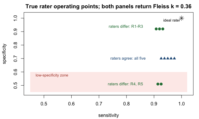
Two panels with one coefficient value and two different internal structures.

This is the case agreement diagnostics miss.

grass_report(Y_shared, verbose = FALSE)
#> GRASS Report Card
#> 
#>   sample      = 5 raters, N = 1000, pi_hat = 0.49
#>   PABAK        = 0.36  ->  56th percentile | quality 0.75-0.85  <- primary
#>   AC1          = 0.36  ->  56th percentile | quality 0.75-0.85
#>   Fleiss kappa = 0.36  ->  56th percentile | quality 0.75-0.85
#>   ICC          = 0.47  ->  61st percentile | quality 0.76-0.85  [distribution-sensitive]
#>   read: this panel's agreement exceeds 56% of what panels in this study context can produce; the data are consistent with panel quality 0.75-0.85.
#>   delta       = 0.00 pp implied-quality spread (aligned)
#>   matched null = (k=5, N=1000, q=0.80): delta_hat sits at percentile 29.2 of the null
#> 
#>   Notes:
#>     - delta_hat is the implied-quality spread over the agreement family (PABAK, mean AC1, Fleiss kappa). ICC is shown but not included in delta_hat; its reference depends on how positive probability is spread across subjects, while the other three depend only on prevalence and quality.
#>     - flag from delta_hat's percentile on the matched null (k=5, N=1000, q=0.80, prev=0.48; 50,000 draws); null interpolated between calibrated grid nodes.
#> 
#>   See `summary(...)` for full panel and CI details.
#>   See `plot(...)` for a surface-position visualization.

The card raises no flag, yet the panel calls about half its subjects positive when the true prevalence is 0.30. Every rater shares the same specificity deficit, so the shared error raises every rater’s positive rate together and no internal comparison can see it. Agreement diagnostics detect raters who disagree with each other, not a panel that is wrong together. Only an external reference standard catches the shared error.

ICC and the subject-prevalence distribution. PABAK, AC1, and Fleiss’ kappa depend only on the positive rate and the rater quality. ICC depends additionally on the full distribution of subject-level positive probabilities; two studies can share a 30% positive rate and differ on whether it comes from obvious positives or borderline cases. The bundled reference covers a 48-point logit-normal grid plus four discrete-mixture profiles, and a panel whose true distribution lies off that grid has its ICC percentile computed against a reference that does not match it. That is why ICC prints a [distribution-sensitive] marker and stays out of delta_hat. The card’s ICC is ICC(1,1), a one-way random-effects model fitted on the logit scale; the package computes no other variant.

Clamping. Every study context has a range of coefficient values it can produce, and an observed value occasionally lands outside that range. No quality produces that value, so the package uses the nearest edge of the range and marks it clamped = TRUE. A clamped reading is a floor or a ceiling rather than a measurement, so grass_report() drops clamped coefficients from delta_hat whenever at least two unclamped ones remain, and reports the clamp in the Notes and in the panel data frame’s clamped and reference_used columns. Clamping is rare. Even at 8% prevalence, near the low edge of the calibrated grid, every coefficient of this five-rater panel inverts cleanly.

Y_edge <- gen_logitnormal(5L, 5L, 1000L,
                          Se = rep(0.85, 5), Sp = rep(0.85, 5), pi = 0.08)
card_edge <- grass_report(Y_edge, bootstrap_B = 50)
card_edge$panel[, c("coefficient", "surface_percentile",
                    "clamped", "reference_used")]
#>    coefficient surface_percentile clamped reference_used
#> 1        pabak           67.75940   FALSE    closed-form
#> 2     mean_ac1           67.67115   FALSE    closed-form
#> 3 fleiss_kappa           67.78800   FALSE    closed-form
#> 4          icc           51.13636   FALSE     fitted-icc

Designs the matrix cannot reveal. The calibration assumes every row is a new subject, and a 0/1 matrix does not say which rows share a patient. Practitioners should avoid stacking the repetitions of one patient as rows, since the repetitions are not independent trials; stacking them overstates the number of subjects and leads to overstated confidence in the reported quality bands. Build one matrix per repetition and compare the cards, or fix one repetition per patient by protocol. When the same patients are scored across sessions over time, each session is a valid panel. One card per session, compared in order, shows whether agreement held over time. Pooling sessions into one number, or splitting disagreement into patient, session, and rater components, is a variance-component analysis and belongs in a mixed model, outside this package.

Study planning and modular functions

Planning a study. Before any data exist, plot_surface() draws a coefficient’s expected-value surface, the value a panel of each quality produces at each prevalence, for a planned rater count and sample size. The observed argument pins a hypothetical value at the planned positive rate. That turns the picture into the planning question: what quality would that value mean in this study, and how far would the same value drift if the prevalence came in differently. The dotted lines mark the quality bands the card uses. A screening study plans three raters, 80 subjects, and a positive rate near 10%, and asks what a Fleiss’ kappa of 0.45 would mean.

plot_surface("fleiss_kappa", pi_hat = 0.10, k = 3, N = 80, observed = 0.45)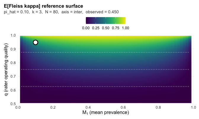

Planning view: Fleiss’ kappa for three raters and 80 subjects, with an observed 0.45 pinned at a 10% positive rate.

At 10% prevalence the pinned 0.45 implies a panel near quality 0.95. The same 0.45 at balanced prevalence would imply a panel near 0.84, because the surface falls away from 50% on both sides. A protocol that fixes a kappa target without fixing the prevalence it applies to has fixed nothing. PABAK’s surface for the same study is flat across prevalence, which is why it is the primary coefficient at moderate prevalence.

plot_surface("pabak", pi_hat = 0.10, k = 3, N = 80, observed = 0.45)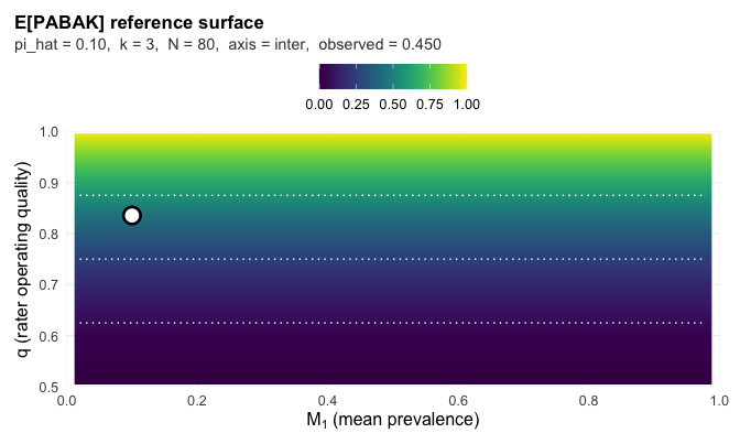

Planning view: PABAK for the same study, with the same observed 0.45 pinned.

The same question with a number instead of a picture: position_on_surface() takes the hypothetical value and the planned study context, with no rating matrix, and returns the implied quality, its percentile, and the consistency band the planned study would give. The metric names are "pabak", "mean_ac1", "fleiss_kappa", and "icc". In a script, assign and print() this result and the plots above, as with the card.

position_on_surface(0.45, "fleiss_kappa", pi_hat = 0.10, k = 3, N = 80)
#> grass surface-position report
#>   metric               : fleiss_kappa
#>   observed value       : 0.450
#>   design (pi_hat,k,N)  : (0.100, 3, 80)
#>   implied quality q_hat: 0.948 +/- 0.019
#>   percentile           : 90.2 (of the achievable range in this study context)
#>   consistency band     : consistent with panel quality 0.90-0.99 (95%)

Each stage of grass_report() on its own.

position_on_surface(ratings = Y1, metric = "pabak")
#> grass surface-position report
#>   metric               : pabak
#>   observed value       : 0.537
#>   design (pi_hat,k,N)  : (0.237, 5, 1000)
#>   implied quality q_hat: 0.866 +/- 0.005
#>   percentile           : 73.9 (of the achievable range in this study context)
#>   consistency band     : consistent with panel quality 0.85-0.90 (95%)
#>   notes                :
#>     - Consistency band narrower than the calibrated q-grid spacing; endpoints interpolated within one grid gap.

position_on_surface() returns the percentile, the band, the implied quality, and, for one coefficient, its position within the sampling distribution at every calibrated quality level, the profile behind the band.

check_asymmetry(ratings = Y1)
#> GRASS panel asymmetry diagnostic
#> 
#>   delta_hat = 0.0 pp  (spread of the implied panel qualities)
#>   flag      = aligned  (36.4 percentile of matched null: k=5, N=1000, q=0.87)
#> 
#>   panel:
#>     coefficient        observed   implied q   pooled pctile   in delta_hat
#>     pabak              0.54       0.866       73.9            yes
#>     mean_ac1           0.64       0.866       73.9            yes
#>     fleiss_kappa       0.36       0.866       73.9            yes
#>     icc                0.48       0.822       62.5            no [distribution-sensitive]
#> 
#>   Surface caveats:
#>     - Consistency band narrower than the calibrated q-grid spacing; endpoints interpolated within one grid gap.
#>     - ICC reference: a logit-normal profile fitted to the ratings (mu=-1.775, tau2=3.089) was matched to the nearest calibrated profile (mu=-1.386, tau2=4.0000).
#>     - ICC reference: calibrated profile LN_mu=-1.386_tau2=4.0000 at k=5, N=1000 (logit_normal family, mean prevalence 0.300).
#>     - delta_hat is the implied-quality spread over the agreement family (PABAK, mean AC1, Fleiss kappa). ICC is shown but not included in delta_hat; its reference depends on how positive probability is spread across subjects, while the other three depend only on prevalence and quality.
#>     - flag from delta_hat's percentile on the matched null (k=5, N=1000, q=0.87, prev=0.14; 50,000 draws); null interpolated between calibrated grid nodes.

check_asymmetry() returns the spread and its flag without per-rater detail.

pairwise_agreement(Y_split)
#> GRASS Pairwise Reliability
#> 
#>   sample      = 5 raters, N = 1000, pi_hat = 0.47, axis = inter
#> 
#>   Pairwise PABAK (lower triangle = PABAK_ij; upper triangle = surface percentile):
#> 
#>    R1     R2     R3     R4     R5    
#> R1     --   84%    84%    48%    40% 
#> R2   0.71     --   81%    45%    41% 
#> R3   0.70   0.67     --   45%    41% 
#> R4   0.27   0.24   0.25     --   35% 
#> R5   0.21   0.22   0.21   0.17     --
#> 
#>   Per-rater behavior against pooled panel-majority:
#> 
#>  rater Se_tilde Sp_tilde n_pos n_neg n_excl
#>     R1     0.84     0.93   360   457    183
#>     R2     0.85     0.91   352   460    188
#>     R3     0.83     0.92   351   459    190
#>     R4     0.92     0.51   327   581     92
#>     R5     0.88     0.50   330   579     91
#>   (Se_tilde, Sp_tilde are calls vs panel-majority of OTHER raters,
#>    not against external truth. n_excl: subjects with tied majority,
#>    excluded from the per-rater pool.)

pairwise_agreement() returns the pairwise matrix and the majority table for any panel, flagged or not, and is the table to report in place of a panel coefficient when the flag is divergent. latent_class_fit() is what the divergent card runs to produce its latent-class table; called on its own it returns that table for any panel, and at two raters the Hui and Walter bounds, as in Case 3.

Other views of a card.

card1 <- grass_report(Y1, verbose = FALSE)
summary(card1)
#> GRASS Report Card -- summary
#> 
#>   sample       : k = 5 raters, N = 1000, pi_hat = 0.237, axis = inter
#> 
#>   primary coefficient
#>     name         : pabak
#>     observed     : 0.537
#>     percentile   : 73.86 (of the achievable range in this study context)
#>     q_hat        : 0.866
#>     band         : consistent with panel quality 0.85-0.90 (95%)
#> 
#>   delta (cross-coefficient asymmetry)
#>     implied-q spread (pp) : 0.00
#>     flag             : aligned
#>     delta percentile : 36.4 (percentile on the matched null, k=5, N=1000, q=0.87)
#> 
#>   panel (full table)
#>     pabak           observed = 0.537  q_hat = 0.866  pct = 73.86  quality 0.85-0.90              ref = closed-form
#>     mean_ac1        observed = 0.637  q_hat = 0.866  pct = 73.86  quality 0.85-0.90              ref = closed-form
#>     fleiss_kappa    observed = 0.361  q_hat = 0.866  pct = 73.86  quality 0.85-0.90              ref = closed-form
#>     icc             observed = 0.484  q_hat = 0.822  pct = 62.50  quality 0.80-0.85              ref = fitted-icc
#> 
#>   notes
#>     - Consistency band narrower than the calibrated q-grid spacing; endpoints interpolated within one grid gap.
#>     - ICC reference: a logit-normal profile fitted to the ratings (mu=-1.775, tau2=3.089) was matched to the nearest calibrated profile (mu=-1.386, tau2=4.0000).
#>     - ICC reference: calibrated profile LN_mu=-1.386_tau2=4.0000 at k=5, N=1000 (logit_normal family, mean prevalence 0.300).
#>     - delta_hat is the implied-quality spread over the agreement family (PABAK, mean AC1, Fleiss kappa). ICC is shown but not included in delta_hat; its reference depends on how positive probability is spread across subjects, while the other three depend only on prevalence and quality.
#>     - flag from delta_hat's percentile on the matched null (k=5, N=1000, q=0.87, prev=0.14; 50,000 draws); null interpolated between calibrated grid nodes.
#> 
#>   grass version : 0.8.0
#>   timestamp     : 2026-09-06 08:34:59

summary() prints everything behind the card, the full panel with percentiles and bands, every caveat from the surface lookup, the package version, and the timestamp.

head(as.data.frame(card1), 5)
#>    coefficient observed_value surface_percentile band_lo band_hi band_open_low
#> 1        pabak      0.5372000           73.86364 0.85125 0.89875         FALSE
#> 2     mean_ac1      0.6372062           73.86364 0.85125 0.89875         FALSE
#> 3 fleiss_kappa      0.3609191           73.86364 0.85125 0.89875         FALSE
#> 4          icc      0.4842583           62.50000 0.80125 0.84875         FALSE
#>   band_open_high     q_hat    se_q_hat clamped reference_used in_delta_hat
#> 1          FALSE 0.8664693 0.005014575   FALSE    closed-form         TRUE
#> 2          FALSE 0.8664471 0.005014821   FALSE    closed-form         TRUE
#> 3          FALSE 0.8664693 0.005014575   FALSE    closed-form         TRUE
#> 4          FALSE 0.8217253 0.002468171   FALSE     fitted-icc        FALSE
#>   is_primary  delta_hat delta_percentile delta_flag matched_null_k
#> 1       TRUE 0.00221665         36.38975    aligned              5
#> 2      FALSE 0.00221665         36.38975    aligned              5
#> 3      FALSE 0.00221665         36.38975    aligned              5
#> 4      FALSE 0.00221665         36.38975    aligned              5
#>   matched_null_N matched_null_q
#> 1           1000      0.8664693
#> 2           1000      0.8664693
#> 3           1000      0.8664693
#> 4           1000      0.8664693

as.data.frame() returns one row per coefficient, for binding many studies’ cards into one table. band_open_low and band_open_high flag a band that reaches the edge of the calibrated quality range; se_q_hat is the standard error of the implied quality, and delta_hat is in quality percentage points, the unit the card prints.

plot(card1)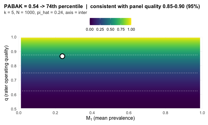

The aligned panel pinned on its PABAK reference surface.

The default plot() places the panel on the expected-value surface in its study context. Other views (type = "thermometer" for the delta_hat gauge, "panel", "intervals", "per_rater", "diagnostic") are documented in ?plot.grass_card.

Reproducibility and references

Every percentile and consistency band above comes from a simulated reference. The bundled calibration holds 44,616 surface cells at 2,000 draws each and 11,616 delta_hat null cells at 50,000 draws each. Study contexts between calibrated cells are handled by interpolation in quality, log sample size, and prevalence; rater count snaps to the nearest calibrated value, so a panel of 17 raters uses the 15-rater reference. The card says so when a snap happens. The simulation programs that produced the bundled references are in the source repository under simulation/. The three case studies are the accompanying paper’s worked examples, regenerated from the same seeds.

• Semmel, A. & Gidaro, R. (2026). A context-conditioned reporting convention for rater reliability on binary outcomes. (Working paper.) The package is the computational companion to this work.
• Byrt, T., Bishop, J. & Carlin, J. B. (1993). Bias, prevalence and kappa. Journal of Clinical Epidemiology 46(5), 423-429.
• Cohen, J. (1960). A coefficient of agreement for nominal scales. Educational and Psychological Measurement 20(1), 37-46.
• Dawid, A. P. & Skene, A. M. (1979). Maximum likelihood estimation of observer error-rates using the EM algorithm. Applied Statistics 28(1), 20-28.
• Fleiss, J. L. (1971). Measuring nominal scale agreement among many raters. Psychological Bulletin 76(5), 378-382.
• Gwet, K. L. (2008). Computing inter-rater reliability and its variance in the presence of high agreement. British Journal of Mathematical and Statistical Psychology 61(1), 29-48.
• Hui, S. L. & Walter, S. D. (1980). Estimating the error rates of diagnostic tests. Biometrics 36(1), 167-171.
• Landis, J. R. & Koch, G. G. (1977). The measurement of observer agreement for categorical data. Biometrics 33(1), 159-174.