GRASS Report Card: a one-call workflow for binary rater reliability

Austin Semmel

Rachel Gidaro

2026-07-03

Abstract

Rater-reliability coefficients drift with prevalence, rater count, and sample size, so a fixed-cutoff label like “substantial agreement” can land on the same panel and mean different things. This package replaces fixed cutoffs with a context-conditioned Report Card, computed in one call from the rating matrix alone. The workflow returns four fields: the sample summary, the primary coefficient with its surface percentile, the cross-coefficient asymmetry diagnostic, and (when the panel disagrees with itself) a per-rater latent-class fit.

What’s new in 0.6.0

• Krippendorff’s α removed from the Report Card and δ̂ (0.6.0): in the binary fully-crossed designs this package targets, α coincides with Fleiss’ κ asymptotically (median absolute difference 0.00024 across the 10,140-cell calibration grid), so its row added no information and its small-sample deviation could tip borderline δ̂ readings across a threshold on noise alone. δ̂ is now the percentile spread over PABAK, mean AC1, and Fleiss’ κ; the bundled thresholds hold for the 3-coefficient spread (sub-pp shift, within MC-SE). obs_krippendorff_alpha() is exported for anyone needing the value, and position_on_surface(metric = "krippendorff_a") still positions it on its closed-form reference.
• Legacy pre-0.2.0 API removed (0.6.0): grass_format_report(), grass_methods(), grass_report_by(), and the grass_result methods. See NEWS.md.

Full release history, including the 0.5.x sysdata corrections, is in NEWS.md.

1. The headline call

The entire workflow is three lines: load the package, pass an N x k binary rating matrix, print the result.

library(grassr)
set.seed(2026)

# Tiny demo: 5 raters, 200 subjects, modest agreement.
truth <- rbinom(200, 1, 0.30)
Y <- sapply(1:5, function(j) {
  ifelse(truth == 1, rbinom(200, 1, 0.85), rbinom(200, 1, 0.15))
})

grass_report(ratings = Y)
#> GRASS Report Card
#> 
#>   sample      = 5 raters, N = 200, pi_hat = 0.34
#>   PABAK        = 0.47  ->  27th percentile  (decisive)  <- primary
#>   AC1          = 0.52  ->  26th percentile
#>   Fleiss kappa = 0.41  ->  31st percentile
#>   ICC          = 0.53  ->  50th percentile  [distribution-sensitive]
#>   delta       = 4.7 pp (aligned)
#>   thresholds  = (9.25, 10.75) [calibrated at this (k, N)]
#> 
#>   Notes:
#>     - Fitted-ICC F_key picked via glmer: mu_hat=-1.039, tau2_hat=3.669 -> F_key tau2=4.0000, mu=-0.847.
#>     - Fitted-ICC reference (GLMM-gap corrected) at F_key=LN_mu=-0.847_tau2=4.0000, k=5, N=200 (family=logit_normal, M1=0.374).
#> 
#>   See `summary(...)` for full panel and CI details.
#>   See `plot(...)` for a surface-position visualization.

Each block in the printed Report Card means something specific:

• sample describes the study: rater count k, subject count N, and the observed positive rate pi_hat = mean(Y).
• The primary coefficient line (e.g. PABAK = 0.41 -> 95th pct (decisive)) shows the observed value, where it lands on the reference surface for this study’s (k, N, pi_hat), and the confidence qualifier (decisive / moderate / weak) reflecting the local envelope width. The percentile is the categorical score; no four-way labeled band sits between the percentile and the reader.
• delta is the cross-coefficient percentile spread in pp across the agreement family (PABAK, AC1, Fleiss kappa; ICC excluded by construction). The caution and divergent cuts are size-α calibrated per (k, N) (delta_thresholds_lookup); at the modal applied design (k = 5, N = 200) the pair is (9.25, 10.75) pp. Below the caution cut the panel is aligned and the primary coefficient is safe to cite; above the divergent cut the panel- aggregate is suppressed in favor of the pairwise PABAK matrix and per-rater pooled-reference Se/Sp.

2. A symmetric panel (the easy case)

Five raters with the same accuracy (Se = Sp = 0.85) on a moderate-prevalence binary task. The panel should land in the aligned tier: every coefficient agrees about where the panel sits, so a single number is enough.

set.seed(29)
N <- 200; k <- 5
truth <- rbinom(N, 1, 0.30)
Y_sym <- sapply(1:k, function(j) {
  ifelse(truth == 1, rbinom(N, 1, 0.85), rbinom(N, 1, 0.15))
})

card_sym <- grass_report(ratings = Y_sym)
card_sym
#> GRASS Report Card
#> 
#>   sample      = 5 raters, N = 200, pi_hat = 0.35
#>   PABAK        = 0.41  ->  95th percentile  (decisive)  <- primary
#>   AC1          = 0.46  ->  94th percentile
#>   Fleiss kappa = 0.36  ->  95th percentile
#>   ICC          = 0.46  ->  50th percentile  [distribution-sensitive]
#>   delta       = 1.2 pp (aligned)
#>   thresholds  = (9.25, 10.75) [calibrated at this (k, N)]
#> 
#>   Notes:
#>     - Fitted-ICC F_key picked via glmer: mu_hat=-0.877, tau2_hat=2.801 -> F_key tau2=4.0000, mu=-0.847.
#>     - Fitted-ICC reference (GLMM-gap corrected) at F_key=LN_mu=-0.847_tau2=4.0000, k=5, N=200 (family=logit_normal, M1=0.374).
#> 
#>   See `summary(...)` for full panel and CI details.
#>   See `plot(...)` for a surface-position visualization.

Note three things:

1. The flag is aligned (delta = 1.2 pp, well below the 9.25-pp caution threshold). One coefficient is safe to cite.
2. Only the primary coefficient prints (PABAK, picked automatically by the (k, pi_hat) rule from Table 2 of the paper). The full panel of four coefficients is still computed and stored on the object; it is just not the headline.
3. The qualifier (decisive) is calibrated, not inherited from a fixed-band convention: it is the bootstrap probability that the modal surface region survives perturbation of (q_hat, pi_hat), mapped to decisive / moderate / weak at 0.90 / 0.60. A four-band label is computed and stored on the object for programmatic use; the printed headline carries the percentile and the qualifier only.

3. A divergent panel

Now the paper’s divergent worked example (the op_strong profile): five raters with alternating per-rater bias direction at balanced prevalence. Three raters lean toward over-calling (Se = 0.95, Sp = 0.75); two lean toward under-calling (Se = 0.75, Sp = 0.95). The asymmetry is severe per rater but cancels in the panel-aggregate marginals, so each agreement coefficient returns roughly the same observed value, yet their inversions onto the (symmetric-DGP) reference surfaces split across percentiles. This is the configuration where the headline grass_report flag flips from a single coherent reading to a per-rater diagnostic.

set.seed(6)
N <- 1000; k <- 5
# Alternating per-rater Se/Sp asymmetry: R1, R3, R5 favor sensitivity;
# R2, R4 favor specificity. Subject-level positive probabilities are
# logit-normal around balanced prevalence (the paper's divergent DGP).
Se <- c(0.95, 0.75, 0.95, 0.75, 0.95)
Sp <- c(0.75, 0.95, 0.75, 0.95, 0.75)
p_i   <- plogis(rnorm(N, qlogis(0.50), sqrt(0.25)))
truth <- rbinom(N, 1L, p_i)
Y_div <- matrix(0L, N, k)
for (j in seq_len(k)) {
  Y_div[, j] <- rbinom(N, 1L, ifelse(truth == 1L, Se[j], 1 - Sp[j]))
}

card_div <- grass_report(ratings = Y_div, bootstrap_B = 200)
card_div
#> GRASS Report Card
#> 
#>   sample      = 5 raters, N = 1000, pi_hat = 0.50
#>   PABAK         = 0.49  ->  40th percentile  <- primary
#>   AC1           = 0.49  ->  58th percentile
#>   Fleiss kappa  = 0.49  ->  41st percentile
#>   ICC           = 0.62  ->  50th percentile  [distribution-sensitive]
#>   panel-agg.  = suppressed (divergent)
#>   delta       =  18 pp (divergent)
#>   thresholds  = (8.50, 9.75) [calibrated at nearest grid cell (snapped)]
#> 
#>   pairwise PABAK / surface percentile (lower / upper):
#>     R1     R2     R3     R4     R5    
#>   R1    --     25%    79%    43%    98% 
#>   R2    0.47   --     97%    90%    17% 
#>   R3    0.51   0.41   --     98%    96% 
#>   R4    0.48   0.52   0.42   --     62% 
#>   R5    0.55   0.46   0.54   0.50   --  
#> 
#>   per-rater vs panel-majority of OTHER raters (pooled-reference):
#>     R1   Se_tilde = 0.94  Sp_tilde = 0.77  (n_pos = 434, n_neg = 471, excl = 95)
#>     R2   Se_tilde = 0.71  Sp_tilde = 0.95  (n_pos = 466, n_neg = 439, excl = 95)
#>     R3   Se_tilde = 0.95  Sp_tilde = 0.71  (n_pos = 433, n_neg = 485, excl = 82)
#>     R4   Se_tilde = 0.74  Sp_tilde = 0.95  (n_pos = 468, n_neg = 441, excl = 91)
#>     R5   Se_tilde = 0.96  Sp_tilde = 0.78  (n_pos = 428, n_neg = 476, excl = 96)
#> 
#>   per-rater (latent-class fit; alongside pairwise):
#>     R1   Se = 0.95  (0.23, 0.97)   Sp = 0.78  (0.06, 0.82)
#>     R2   Se = 0.73  (0.05, 0.77)   Sp = 0.95  (0.29, 0.97)
#>     R3   Se = 0.96  (0.29, 0.97)   Sp = 0.72  (0.05, 0.76)
#>     R4   Se = 0.75  (0.05, 0.79)   Sp = 0.95  (0.26, 0.97)
#>     R5   Se = 0.96  (0.22, 0.98)   Sp = 0.78  (0.04, 0.82)
#> 
#>   Notes:
#>     - (k = 5, N = 1000) has no fully-calibrated threshold pair on the grid (or is off-grid); using nearest fully-calibrated cell (k = 5, N = 500).
#>     - Fitted-ICC F_key picked via glmer: mu_hat=0.005, tau2_hat=5.278 -> F_key tau2=4.0000, mu=0.000.
#>     - Fitted-ICC reference (GLMM-gap corrected) at F_key=LN_mu=+0.000_tau2=4.0000, k=5, N=1000 (family=logit_normal, M1=0.500).
#> 
#>   See `summary(...)` for full panel and CI details.
#>   See `plot(...)` for a surface-position visualization.

The flag is divergent: the cross-coefficient percentile spread clears the divergent threshold printed on the card (9.75 pp, snapped from the nearest calibrated cell) even though the three agreement coefficients (PABAK, AC1, Fleiss kappa) all sit near the same observed value. Three things change in the printed output:

1. The full panel of percentiles prints, not just the primary, so the reader can see that AC1 separates from the kappa-family coefficients.
2. The band is suppressed. Picking a single number from a panel whose coefficients disagree on the surface position would hide the asymmetry.
3. The per-rater table appears. A latent-class fit (Dawid-Skene EM at k >= 3, Hui-Walter bounds at k = 2) recovers each rater’s sensitivity and specificity with bootstrap confidence intervals. The recovered estimates pin the panel’s structure: R1, R3, R5 land near (Se, Sp) = (0.95, 0.75), R2, R4 near (0.75, 0.95). The bootstrap CIs are wide because the latent-class likelihood becomes ridge-flat near balanced prevalence and the bootstrap resamples both the correct mode and its label-switched counterpart; the point estimates pin the local mode, but without external orientation the practitioner cannot assert from the rating matrix alone which raters are over- versus under-callers.

Pairwise reliability under the divergent flag

When the panel is divergent the framework’s recommended primary deliverable is pairwise_agreement(): a k x k matrix of pairwise PABAK values, each placed on the k = 2 reference surface at the pair’s observed marginal, plus per-rater behavior against the panel-majority of the other k - 1 raters as a proxy reference. The pairwise matrix exposes the panel’s structure directly, and the pooled-reference per-rater table avoids the latent-class identifiability problem (label-switching is moot because the “reference” is the observable panel majority, not a latent class).

pw <- pairwise_agreement(Y_div)
pw
#> GRASS Pairwise Reliability
#> 
#>   sample      = 5 raters, N = 1000, pi_hat = 0.50, tau2_hat = 0.122, axis = inter
#> 
#>   Pairwise PABAK (lower triangle = PABAK_ij; upper triangle = surface percentile):
#> 
#>    R1     R2     R3     R4     R5    
#> R1     --   25%    79%    43%    98% 
#> R2   0.47     --   97%    90%    17% 
#> R3   0.51   0.41     --   98%    96% 
#> R4   0.48   0.52   0.42     --   62% 
#> R5   0.55   0.46   0.54   0.50     --
#> 
#>   Per-rater behavior against pooled panel-majority:
#> 
#>  rater Se_tilde Sp_tilde n_pos n_neg n_excl
#>     R1     0.94     0.77   434   471     95
#>     R2     0.71     0.95   466   439     95
#>     R3     0.95     0.71   433   485     82
#>     R4     0.74     0.95   468   441     91
#>     R5     0.96     0.78   428   476     96
#>   (Se_tilde, Sp_tilde are calls vs panel-majority of OTHER raters,
#>    not against external truth. n_excl: subjects with tied majority,
#>    excluded from the per-rater pool.)

Read the per-rater table: with R1, R3, R5 favoring sensitivity and R2, R4 favoring specificity, the pooled-reference estimates pin each rater’s bias direction without ambiguity. R1’s Se_tilde is high (calls true positives at panel-majority rate) while Sp_tilde is lower (calls panel-majority negatives less reliably): the over-caller signature. R2 shows the mirror: low Se_tilde, high Sp_tilde. The latent-class fit’s wide bootstrap CIs in the paper’s divergent example had to live with the label-switched mode; the pooled-reference per-rater table sidesteps that ambiguity.

The pairwise PABAK matrix lower triangle shows the actual pairwise agreements; the upper triangle shows surface percentiles at each pair’s observed marginal. Note that the same PABAK value can land at different surface percentiles across pairs because each pair sees a different pi_hat_ij; the divergent flag is exposing exactly this prevalence-by-pair structure that a panel-aggregate summary would have averaged away.

4. Layered access

Every field beneath the printed Report Card is available on demand.

summary(card_sym)
#> GRASS Report Card -- summary
#> 
#>   sample       : k = 5 raters, N = 200, pi_hat = 0.354, axis = inter
#>   tau2_hat     : 0.083
#> 
#>   primary coefficient
#>     name         : pabak
#>     observed     : 0.414
#>     percentile   : 95.42 pp
#>     band         : Strong
#>     qualifier    : decisive
#> 
#>   delta (cross-coefficient asymmetry)
#>     delta_hat    : 1.20 pp
#>     flag         : aligned
#>     thresholds   : caution = 9.25, divergent = 10.75
#> 
#>   panel (full table)
#>     pabak           observed = 0.414  pct = 95.42 pp  band = Strong       qualifier = decisive
#>     mean_ac1        observed = 0.460  pct = 94.22 pp  band = Strong       qualifier = decisive
#>     fleiss_kappa    observed = 0.359  pct = 94.67 pp  band = Strong       qualifier = decisive
#>     icc             observed = 0.464  pct = 50.00 pp  band = Strong       qualifier = decisive
#> 
#>   notes
#>     - Fitted-ICC F_key picked via glmer: mu_hat=-0.877, tau2_hat=2.801 -> F_key tau2=4.0000, mu=-0.847.
#>     - Fitted-ICC reference (GLMM-gap corrected) at F_key=LN_mu=-0.847_tau2=4.0000, k=5, N=200 (family=logit_normal, M1=0.374).
#> 
#>   grass version : 0.6.1
#>   timestamp     : 2026-07-03 13:30:16

summary() is the audit view: full panel of coefficients with percentiles and bands, all caveats from the surface lookup, the GRASS version, the timestamp. Use it when you want to see what the headline hides.

head(as.data.frame(card_sym), 5)
#>    coefficient observed_value surface_percentile   band qualifier
#> 1        pabak      0.4140000           95.41694 Strong  decisive
#> 2     mean_ac1      0.4601604           94.21535 Strong  decisive
#> 3 fleiss_kappa      0.3593780           94.66860 Strong  decisive
#> 4          icc      0.4641657           50.00000 Strong  decisive
#>   band_probability_modal     q_hat    se_q_hat clamped reference_used
#> 1                      1 0.8217138 0.013797700   FALSE    closed-form
#> 2                      1 0.8217650 0.013796793   FALSE    closed-form
#> 3                      1 0.8217138 0.013797700   FALSE    closed-form
#> 4                      1 0.8075234 0.005569156   FALSE     fitted-icc
#>   in_delta_hat is_primary
#> 1         TRUE       TRUE
#> 2         TRUE      FALSE
#> 3         TRUE      FALSE
#> 4        FALSE      FALSE

as.data.frame() is the tidy view: one row per coefficient with observed_value, surface_percentile, band, qualifier, and is_primary. Use it when you want to bind many studies’ Report Cards into one table for a meta-analysis or to feed the panel into another analysis pipeline.

plot(card_sym)                       # default: surface with observation pinned
#> Warning: The following aesthetics were dropped during statistical transformation: fill.
#> ℹ This can happen when ggplot fails to infer the correct grouping structure in
#>   the data.
#> ℹ Did you forget to specify a `group` aesthetic or to convert a numerical
#>   variable into a factor?
#> Warning: Removed 120 rows containing missing values or values outside the scale range
#> (`geom_raster()`).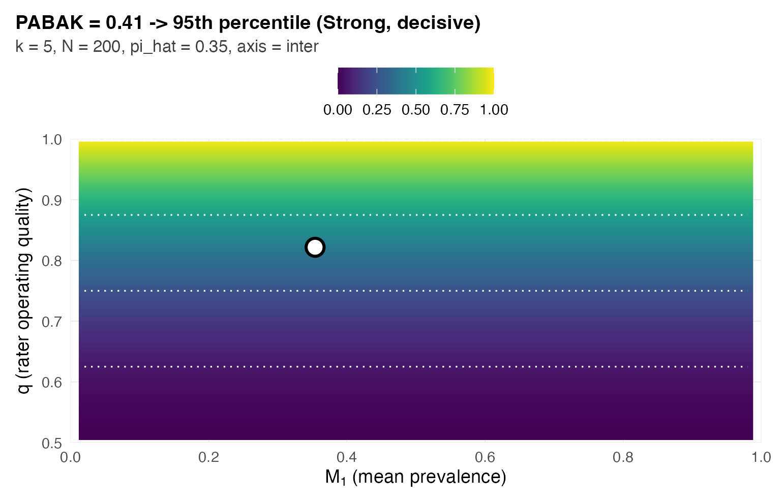

plot(card_sym, type = "thermometer") # delta_hat thermometer
#> Warning: Removed 1 row containing missing values or values outside the scale range
#> (`geom_rect()`).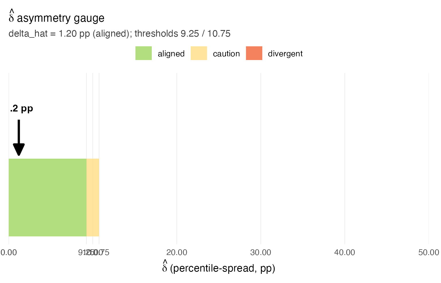

The default plot() view is a heatmap of the expected primary coefficient over (M_1, q) at the study’s (k, N), with a single point pinned at the observed coordinates. The thermometer view isolates delta_hat against the caution and divergent thresholds; useful when the question is “is the panel stable enough to cite a single number?”. Additional views (type = "panel" for the cross-coefficient spread, type = "intervals" for forest-style CIs, type = "per_rater" for the divergent-branch per-rater forest, type = "diagnostic" for a combined patchwork) are documented in ?plot.grass_card.

5. Granular building blocks

For users who want lower-level control, three of the internals grass_report() calls are exported:

position_on_surface(ratings = Y_sym, metric = "pabak")
#> grass surface-position report (Target-2 reporting convention)
#>   metric               : pabak
#>   observed value       : 0.414
#>   design (pi_hat,k,N)  : (0.354, 5, 200)
#>   q_hat (scaffold)     : 0.822 +/- 0.014
#>   surface percentile   : 0.954
#>   band probabilities   :
#>     Poor       0.000
#>     Moderate   0.000
#>     Strong     1.000 <- modal
#>     Excellent  0.000
#>   label                : Strong (decisive)
#>   sampling method      : empirical

position_on_surface() does the surface lookup for a single coefficient and returns the percentile, band, and band-probability vector.

check_asymmetry(ratings = Y_sym)
#> GRASS panel asymmetry diagnostic
#> 
#>   delta_hat = 1.2 pp
#>   flag      = aligned  (< 9.2)
#> 
#>   panel:
#>     coefficient        observed   percentile (pp)   in delta_hat
#>     pabak              0.41       95.4             yes
#>     mean_ac1           0.46       94.2             yes
#>     fleiss_kappa       0.36       94.7             yes
#>     icc                0.46       50.0             no [distribution-sensitive]
#> 
#>   Surface caveats:
#>     - Fitted-ICC F_key picked via glmer: mu_hat=-0.877, tau2_hat=2.801 -> F_key tau2=4.0000, mu=-0.847.
#>     - Fitted-ICC reference (GLMM-gap corrected) at F_key=LN_mu=-0.847_tau2=4.0000, k=5, N=200 (family=logit_normal, M1=0.374).
#>     - delta_hat is computed over the agreement family (PABAK, AC1, Fleiss, alpha). ICC is reported on the panel but does not enter delta_hat (v0.5.0 scope: ICC's reference surface depends on the full subject-prevalence distribution F and does not share the (q, pi_+) sufficient statistic the agreement family does).

check_asymmetry() returns the cross-coefficient percentile spread and the (aligned / caution / divergent) flag without computing per-rater detail. Cheap when you want only the diagnostic.

latent_class_fit(ratings = Y_div, B = 200)
#> grass latent-class fit
#>   method        : dawid_skene_em
#>   raters (k)    : 5
#>   bootstrap B   : 200
#>   converged     : TRUE
#>   iterations    : 10
#>   prevalence_hat: 0.475
#>   log-likelihood: -2504.371
#>   per-rater
#>     R1    Se = 0.950  (0.201, 0.970)   Sp = 0.783  (0.050, 0.817)
#>     R2    Se = 0.729  (0.042, 0.770)   Sp = 0.953  (0.259, 0.973)
#>     R3    Se = 0.956  (0.262, 0.973)   Sp = 0.718  (0.036, 0.764)
#>     R4    Se = 0.750  (0.044, 0.784)   Sp = 0.949  (0.259, 0.965)
#>     R5    Se = 0.962  (0.206, 0.980)   Sp = 0.781  (0.038, 0.812)

latent_class_fit() produces the per-rater Se/Sp table directly, with Dawid-Skene EM and a nonparametric bootstrap CI at k >= 3.

6. Two-rater binary case (k = 2)

The headline call works at k = 2 with no signature change:

set.seed(42)
N <- 200
truth <- rbinom(N, 1, 0.30)
Y_k2 <- cbind(
  ifelse(truth == 1, rbinom(N, 1, 0.85), rbinom(N, 1, 0.15)),
  ifelse(truth == 1, rbinom(N, 1, 0.85), rbinom(N, 1, 0.15))
)

grass_report(ratings = Y_k2)
#> GRASS Report Card
#> 
#>   sample      = 2 raters, N = 200, pi_hat = 0.39
#>   PABAK  = 0.50  ->  56th percentile  (decisive)  <- primary
#>   AC1    = 0.52  ->  57th percentile
#>   delta       = 0.4 pp (aligned)
#>   thresholds  = (8.25, 9.75) [calibrated at nearest grid cell (snapped)]
#> 
#>   Notes:
#>     - (k = 2, N = 200) has no fully-calibrated threshold pair on the grid (or is off-grid); using nearest fully-calibrated cell (k = 3, N = 200).
#> 
#>   See `summary(...)` for full panel and CI details.
#>   See `plot(...)` for a surface-position visualization.

When the panel goes divergent at k = 2, per-rater Se and Sp are not point-identified from the rating matrix alone (there is one fewer constraint than parameter). The latent-class fit returns Hui-Walter bounds rather than point estimates:

latent_class_fit(ratings = Y_k2, B = 200)
#> grass latent-class fit
#>   method        : hui_walter
#>   raters (k)    : 2
#>   bootstrap B   : 200
#>   per-rater
#>     R1    Se in [0.395, 1.000]   Sp in [0.605, 1.000]   (bounds)
#>     R2    Se in [0.385, 1.000]   Sp in [0.615, 1.000]   (bounds)
#> 
#>   Note: at k = 2, per-rater Se/Sp are not point-identified
#>         without external information. The intervals are
#>         Hui-Walter (1980) inequality bounds, not point
#>         estimates with sampling uncertainty.

The bounds carry the same meaning as the k >= 3 point estimates: an honest representation of what the data say about each rater. At k = 2 that is a range; at k >= 3 it is a point with uncertainty.

7. Surface-envelope clamp (an edge case worth knowing about)

delta_hat measures cross-coefficient surface-percentile spread. If one of the panel’s coefficients reports an observed value that falls outside the achievable range of its reference surface at the study’s design (pi_hat, k, N), the inversion to q_hat clamps to the surface boundary and the percentile lands at exactly 0 or 100. Since v0.2.2, check_asymmetry() and grass_report() exclude such clamped coefficients from delta_hat whenever at least two unclamped coefficients remain — otherwise a single clamped coefficient could inflate the spread by 100 pp and fire a false divergent flag.

The most common trigger is ICC at N > 200. The bundled fitted-ICC reference is calibrated at N in {50, 200}; beyond that, the function falls back to the oracle ICC reference (closed-form, no GLMM-gap correction), which over-predicts the practitioner’s glmer-fit ICC and clamps the percentile to 0:

# A panel where ICC clamps but the three agreement coefficients align.
set.seed(5)
N <- 1000L; k <- 5L
mu_logit <- qlogis(0.08)
p_i <- plogis(rnorm(N, mu_logit, sqrt(0.25)))
truth <- rbinom(N, 1, p_i)
Y_clamp <- matrix(0L, N, k)
for (j in seq_len(k)) {
  Y_clamp[, j] <- rbinom(N, 1, ifelse(truth == 1, 0.85, 0.15))
}
card_clamp <- grass_report(Y_clamp, bootstrap_B = 50)
card_clamp
#> GRASS Report Card
#> 
#>   sample      = 5 raters, N = 1000, pi_hat = 0.21
#>   PABAK        = 0.49  ->  46th percentile  (decisive)  <- primary
#>   AC1          = 0.62  ->  46th percentile
#>   Fleiss kappa = 0.23  ->  47th percentile
#>   ICC          = 0.33  ->  50th percentile  [distribution-sensitive]
#>   delta       =   1 pp (aligned)
#>   thresholds  = (8.50, 9.75) [calibrated at nearest grid cell (snapped)]
#> 
#>   Notes:
#>     - (k = 5, N = 1000) has no fully-calibrated threshold pair on the grid (or is off-grid); using nearest fully-calibrated cell (k = 5, N = 500).
#>     - Fitted-ICC F_key picked via glmer: mu_hat=-1.716, tau2_hat=1.633 -> F_key tau2=1.0000, mu=-1.386.
#>     - Fitted-ICC reference (GLMM-gap corrected) at F_key=LN_mu=-1.386_tau2=1.0000, k=5, N=1000 (family=logit_normal, M1=0.239).
#> 
#>   See `summary(...)` for full panel and CI details.
#>   See `plot(...)` for a surface-position visualization.

The printed Report Card surfaces the clamp in two places: the Notes section names which coefficient was excluded and why, and under the divergent flag the panel display marks each clamped coefficient row with [clamped - excluded from delta]. The panel data.frame on the returned object also carries a clamped logical column for programmatic inspection:

card_clamp$panel[, c("coefficient", "surface_percentile",
                     "band", "clamped")]
#>    coefficient surface_percentile   band clamped
#> 1        pabak           46.27444 Strong   FALSE
#> 2     mean_ac1           45.50669 Strong   FALSE
#> 3 fleiss_kappa           46.52487 Strong   FALSE
#> 4          icc           50.00000 Strong   FALSE

The trade-off: a coefficient with no calibrated reference at the user’s design contributes nothing to the diagnostic. The benefit: when delta_hat does fire divergent, it reflects genuine cross-coefficient surface-percentile disagreement rather than an envelope artifact. If the clamp is cosmetic (the three agreement coefficients align cleanly without ICC), the Report Card’s verdict is the right one. If clamping coincides with a real divergent panel (rare but possible), the Notes line and the clamped column let the practitioner audit which coefficients contributed to the diagnostic.

8. Prospective design: plot_surface()

The Report Card workflow assumes you already have a rating matrix. For study design — “what would my reference surface look like at k = 8, N = 200, pi_hat = 0.30 before I collect data?” — use the new plot_surface() entry point.

The bare call shows the closed-form expected value of a coefficient across the entire surface (mean prevalence M_1 × rater operating quality q). Dotted contours overlay equal-spaced reference levels on the q-axis (computational scaffolding for the qualifier; not displayed on the headline Report Card), so the reader can see which combinations of prevalence and rater quality land where:

plot_surface("fleiss_kappa")
#> Warning: The following aesthetics were dropped during statistical transformation: fill.
#> ℹ This can happen when ggplot fails to infer the correct grouping structure in
#>   the data.
#> ℹ Did you forget to specify a `group` aesthetic or to convert a numerical
#>   variable into a factor?
#> Warning: Removed 120 rows containing missing values or values outside the scale range
#> (`geom_raster()`).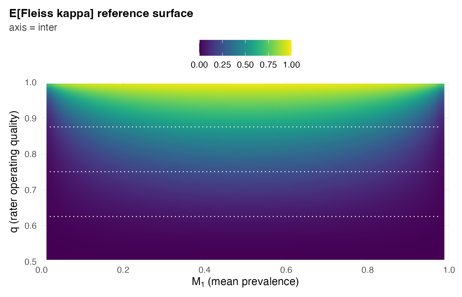

Adding a design context overlays a dashed reference at the planned marginal:

plot_surface("mean_ac1",
             pi_hat = 0.30,
             k      = 8,
             N      = 200)
#> Warning: The following aesthetics were dropped during statistical transformation: fill.
#> ℹ This can happen when ggplot fails to infer the correct grouping structure in
#>   the data.
#> ℹ Did you forget to specify a `group` aesthetic or to convert a numerical
#>   variable into a factor?
#> Warning: Removed 120 rows containing missing values or values outside the scale range
#> (`geom_raster()`).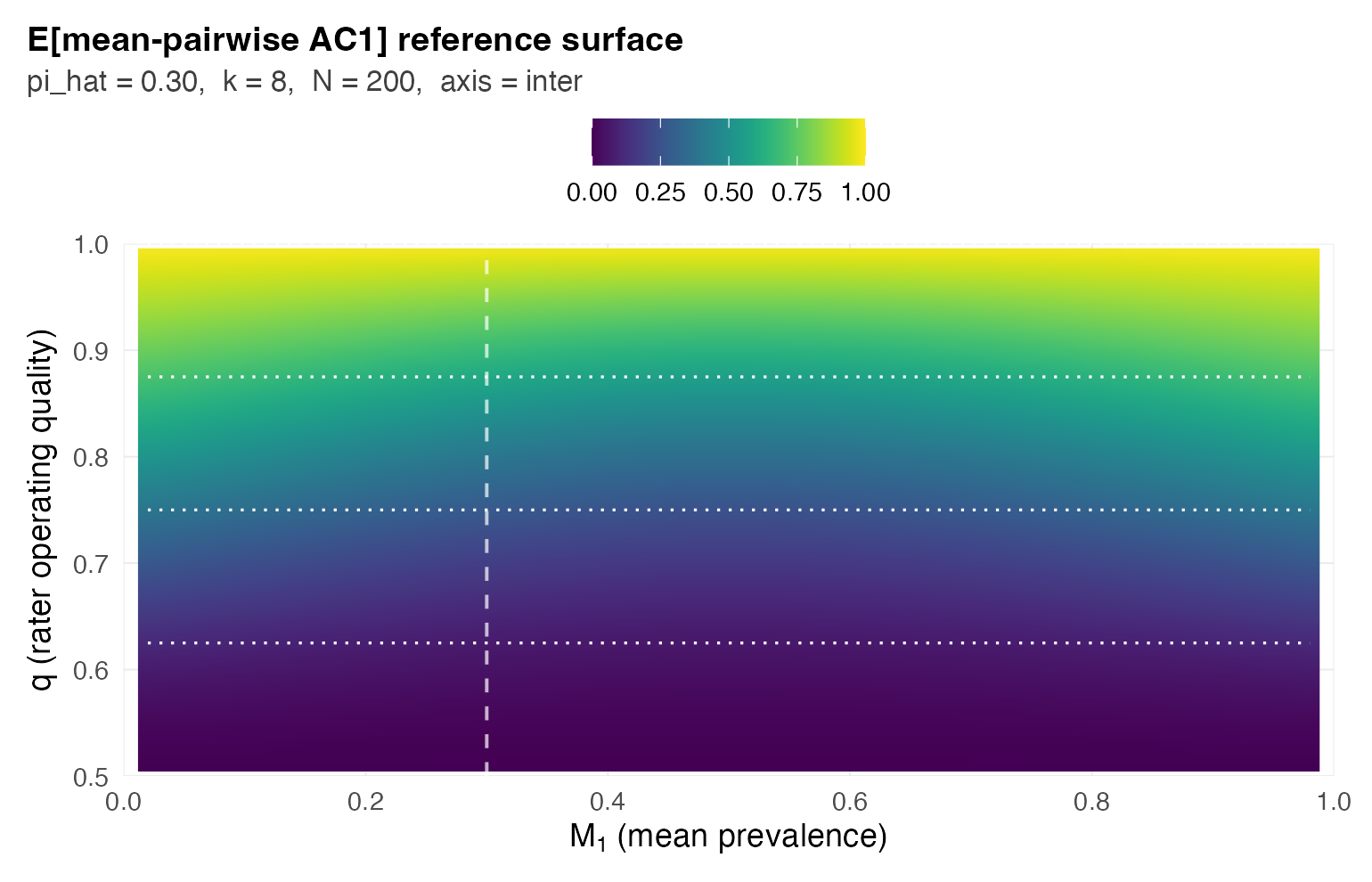

Adding a hypothetical observed value pins a marker at (pi_hat, hat q), where hat q is recovered by closed-form inversion against the reference curve at pi_hat. This answers “if I observe Fleiss kappa = 0.50 in a panel at this design, where on the surface would I sit?”:

plot_surface("fleiss_kappa",
             pi_hat   = 0.30,
             observed = 0.50,
             k        = 8,
             N        = 200)
#> Warning: The following aesthetics were dropped during statistical transformation: fill.
#> ℹ This can happen when ggplot fails to infer the correct grouping structure in
#>   the data.
#> ℹ Did you forget to specify a `group` aesthetic or to convert a numerical
#>   variable into a factor?
#> Warning: Removed 120 rows containing missing values or values outside the scale range
#> (`geom_raster()`).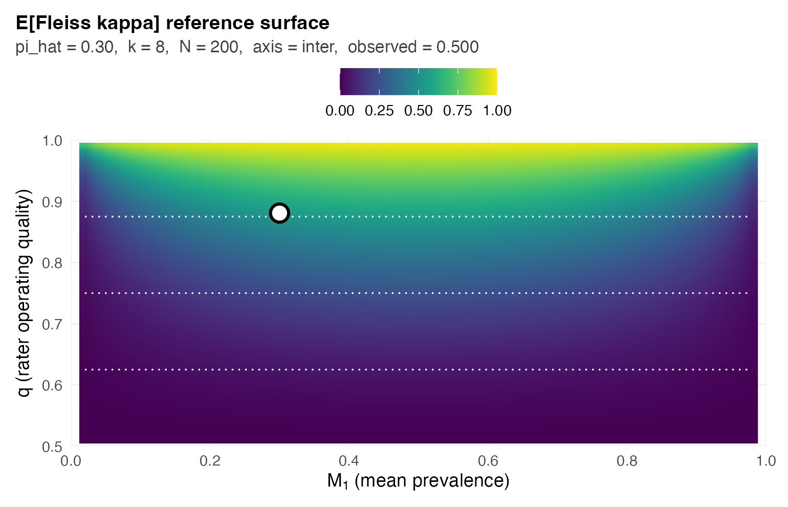

plot_surface() supports the four closed-form non-ICC metrics (PABAK, Fleiss kappa, mean-pairwise AC1, and — although it no longer appears on the Report Card — Krippendorff alpha). ICC surfaces depend on the full subject-prevalence distribution F and the GLMM-gap-corrected fitted reference; for ICC, build a card with grass_report() and use plot.grass_card(type = "surface").

References

• Semmel, A. & Gidaro, R. (2026). GRASS: A context-conditioned reporting convention for binary rater reliability. (Working paper.) The package is the computational companion to this work; the four-field Report Card and the surface-percentile machinery are documented in detail there.
• Hui, S. L. & Walter, S. D. (1980). Estimating the error rates of diagnostic tests. Biometrics 36(1), 167-171. The k = 2 bounds returned by latent_class_fit().
• Dawid, A. P. & Skene, A. M. (1979). Maximum likelihood estimation of observer error-rates using the EM algorithm. Applied Statistics 28(1), 20-28. The k >= 3 EM fit.